Overview of Water Damage in Logs
Waterlogged timber swells, cracks, and develops mold, compromising structural integrity. Moisture infiltration weakens cell walls, causing dimensional instability and decay. Early detection and proper drying mitigate long‑term damage, preserving value and safety. Sustainable practices cut waste
Assessment Before Drying
Before drying, assess the log’s condition. This step ensures the chosen method addresses moisture profile and structural concerns without accelerating damage.
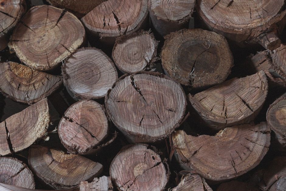
- Visual Inspection: Check for rot, fungal growth, bark integrity, and cracks. Note grain orientation and end‑grain exposure that may retain moisture.
- Moisture Meter Survey: Use a pin‑probe meter to record core, mid‑wood, and outer moisture. Readings above 12 % indicate high core moisture.
- Dimensional Check: Measure dimensions to detect swelling or shrinkage. Check for uneven grain and ensure no cracks form, ends stay.
- Environmental Context: Evaluate ambient temperature, humidity, and airflow around the storage area; High humidity can impede drying, while drafts may cause surface cracking.
- Risk Evaluation: Identify potential hazards such as mold spores, insect infestation, or structural instability that could compromise safety during drying.
Once data is collected, a drying plan is tailored: logs with high core moisture may require a kiln, while surface‑moist logs can be air‑dried with protective stacking. Documentation of initial readings provides a baseline for monitoring progress and validating the effectiveness of the chosen drying technique.
Drying Techniques
Drying logs for water damage requires a blend of traditional and modern methods. The choice hinges on log size, moisture content, and desired finish. Below are the primary techniques:
- Air‑Drying with Protective Stacking: Place logs on a raised platform, ensuring airflow beneath. Stack with end‑grain facing down to shield wet edges. Use breathable materials like burlap or mesh to prevent mold while allowing moisture escape. Place logs on racks to maximize sun exposure. This method reduces energy costs and preserves wood color.
- Solar Kiln Drying: Construct a greenhouse‑style enclosure with south‑facing glazing. Add reflective panels to concentrate heat. Logs are arranged on racks to maximize sun exposure. This method reduces energy costs and preserves wood color.
- Conventional Oven Drying for Small Blanks: Set temperature between 120–140 °F (49–60 °C) and monitor moisture with a probe. Rotate logs every 12–24 h to avoid uneven drying.
- Mechanical Ventilation: Install fans or blowers to circulate air around stacked logs. This speeds moisture removal, especially in humid climates.
- Controlled Humidity Chambers: Maintain relative humidity at 30–40 % and temperature at 70–80 °F (21–27 °C). Logs are placed on racks; moisture is extracted gradually, minimizing shrinkage cracks.
method requires monitoring. Moisture meter checks prevent over‑drying, which can cause warping or splitting. Selecting the right technique ensures logs recover strength stability!!!?!!
Commercial Kiln Services
Professional kiln services offer a controlled environment for removing excess moisture from logs, ensuring uniform drying and preventing defects. These facilities use high‑temperature, low‑humidity chambers that accelerate moisture extraction while maintaining structural integrity. Logs are placed on adjustable racks, allowing air to circulate around each piece. Sensors monitoring temperature and humidity, enabling real‑time adjustments to optimize drying cycles. The process typically begins with an initial “pre‑dry” phase at moderate temperatures to reduce surface moisture, followed by a “core‑dry” phase that targets internal moisture. This staged approach minimizes the risk of cracking, warping, or fungal growth. Commercial kilns can handle large volumes, making them ideal for sawmills, furniture manufacturers, and restoration projects. They also provide detailed moisture‑content reports, allowing clients to track progress and verify compliance with industry standards. By outsourcing to a specialized kiln operator, businesses can achieve consistent quality, reduce energy consumption through efficient heat recovery systems, and free up on‑site resources for other production tasks. Additionally, many kiln operators offer customized drying schedules tailored to specific wood species, desired end‑use, and environmental regulations, ensuring that each log reaches the optimal moisture level for its intended application. The investment in professional kiln drying often pays off through extended product life, enhanced aesthetic appeal, and compliance with safety codes. For anyone looking to preserve the integrity of water‑damaged logs, commercial kiln drying presents a reliable, scalable, and scientifically grounded solution that balances speed, cost, and quality!!
Stacking and Protective Measures
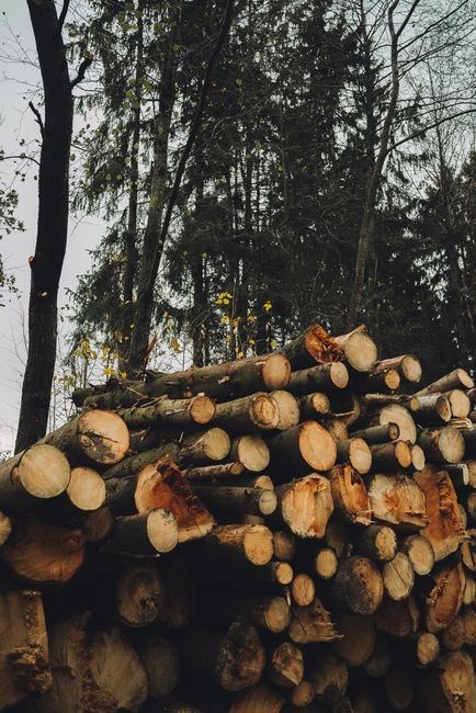
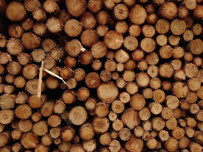
When logs are cut from a freshly felled tree, their ends remain saturated with sap and surface moisture. Proper stacking mitigates cracking and warping by protecting the outer layers while the cores dry. A common method places each log on its end, then stacks the next on top, shielding the exposed end grain of the lower log. This reduces direct air exposure, slowing end‑grain drying and preventing “end‑grain cracks.” Logs can also be laid on a flat, non‑absorbent surface such as plywood or concrete, providing a stable base and consistent airflow. Covering the stack with a breathable tarp or mesh shields from rain and direct sunlight while allowing moisture to escape; For larger volumes, a tiered system with spacers or ventilation gaps ensures uniform airflow around each log. These stacking strategies preserve structural integrity, reduce overall drying time, and create a micro‑environment that balances moisture loss and temperature. By maintaining uniform airflow and preventing moisture pockets, this stacking technique also reduces the risk of fungal growth during the drying period. Logs are stacked cross‑wise to maximize surface area exposure. Spacers like wooden blocks or metal rods create ventilation gaps of 2–3 cm. Hot air circulates, preventing trapped moisture. Logs can be wrapped in moisture‑resistant film during transport, aiding consistent drying. When the stack reaches target moisture, logs are removed slowly to avoid temperature shocks that cause cracking. This method also conserves energy by reducing the need for prolonged kiln operation. It is a cost‑effective solution for small workshops. and saves.
Monitoring Drying Progress
Accurate monitoring ensures logs reach safe moisture levels without over‑drying. Begin with a calibrated moisture meter and record readings at end grain, center, and side. Tag each log for traceability. Log daily data—moisture, ambient temperature, relative humidity, and visual notes—into a spreadsheet or logbook. In kilns, a data logger records chamber temperature and humidity, allowing real‑time adjustments to airflow or heat cycles. Outdoor stacks benefit from a simple weather station to correlate drying rates with environmental conditions. Visual inspections spot early mold or cracking; if moisture drops too quickly, re‑stack or cover the log to slow the rate. If moisture remains high, move the log to a more ventilated area or extend kiln time. Operators also monitor kiln pressure to prevent condensation. Combining quantitative meter data with qualitative observations fine‑tunes drying schedules, reduces energy use, and yields structurally sound logs ready for storage or processing.
Periodic core checks reveal internal gradients missed by surface readings. Cutting a small core and measuring its moisture provides a definitive snapshot of internal conditions, especially for large logs where end grain dries faster than the core. Integrating core data allows targeted heat or adjusted stacking orientation. Documentation of each adjustment ensures repeatability for future batches. When logs reach target moisture—typically 6–8 % for firewood or 12–15 % for structural timber—the final inspection confirms uniformity. Consistent monitoring protects product quality and safeguards the investment in drying equipment and labor. Data logged for trend analysis dailyNow!Today
Documentation and PDF Guides
PDF manuals cover kiln setup, safety, moisture targets, and step‑by‑step drying charts. They include sensor calibration, inspection logs, and templates for record‑keeping. The guide offers stacking, ventilation, and post‑dry treatment best practices daily.
Causes and Effects of Water Damage
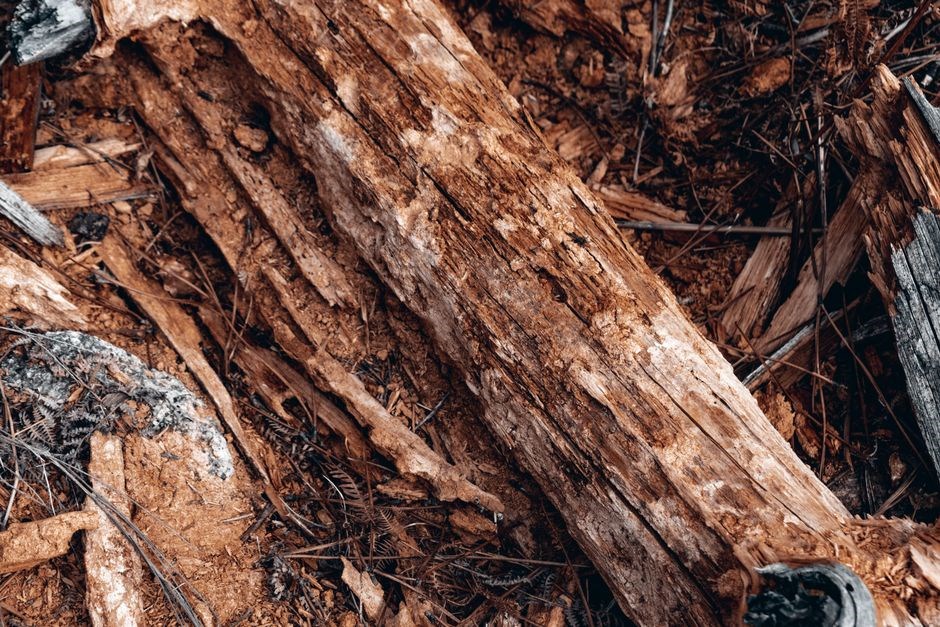
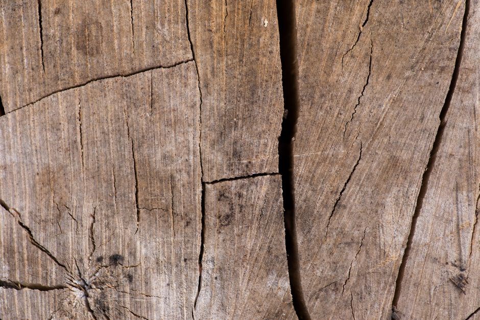
Water infiltration originates from rain, snowmelt, groundwater, or improper storage. Saturated logs expand, causing internal stresses that fracture cell walls. High moisture content fosters fungal growth, accelerating decay and weakening structural bonds. Swelling leads to dimensional instability, warping, and surface cracking. As water evaporates, it leaves voids and reduces density, making the timber prone to impact damage. Mold spores thrive, producing allergens and compromising indoor air quality. Long‑term exposure can result in loss of load‑bearing capacity, rendering the log unsafe for construction or firewood use. Immediate drying reduces these risks, but delayed action allows irreversible damage.
Waterlogged timber often originates from prolonged exposure to saturated soils, especially in low‑lying areas where drainage is poor. The high moisture content not only weakens the cellulose network but also creates a favorable environment for rot fungi such as Phytophthora and Serpula. These organisms degrade lignin, leading to softening and loss of compressive strength. Additionally, water penetration can cause internal stresses that manifest as warping, cupping, and split ends, which compromise load‑bearing capacity. The presence of mold spores also poses health risks, producing allergens and organic degrade indoor air quality. Thus, timely drying is essential to preserve structural integrity and prevent long‑term deterioration.
Visual Inspection Methods
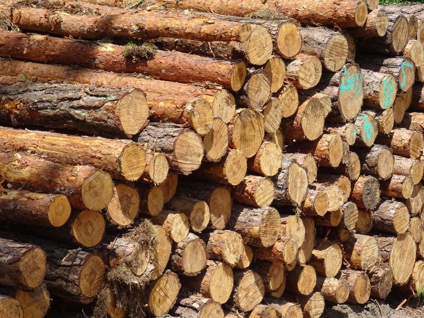
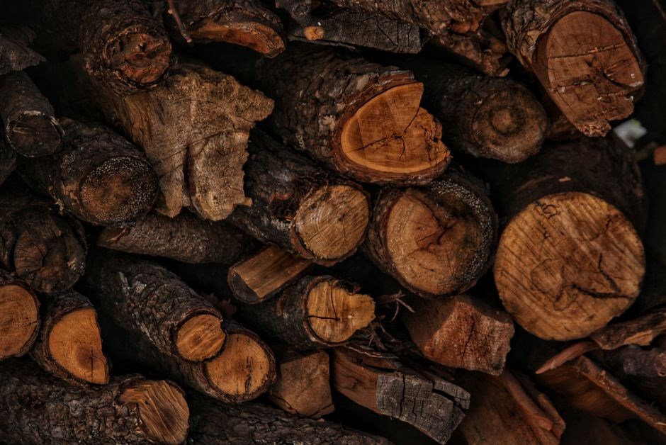
When evaluating logs for moisture damage, start with a thorough visual scan. Look for surface discoloration—green or dark patches indicate high moisture and potential rot. Inspect end grain; a wet end will feel damp, often with a slight sheen, and may show soft spots or mold growth. A good rule of thumb is to run a finger along the surface; a wet log will feel cool and slightly tacky. Use a flashlight to spot hidden cavities or internal decay, especially in the heartwood. Finally, compare the log’s weight to a dry reference; a heavier log suggests retained moisture. Document findings with photos and notes before initiating any drying process.
When performing a visual inspection, start at the base and work upward, noting any unevenness or discoloration that may indicate moisture pockets. Pay special attention to the bark; a wet bark often appears glossy and may have a soft feel. Check for fungal fruiting bodies such as bracket fungi or soft rot, which can be identified by their irregular, spongy texture. Use a magnifying glass to examine the grain for microcracks or delamination. If the log has been stored in a damp environment, look for signs of swelling or warping, especially along the growth rings. Document each observation with a photo, labeling the log number, date, and specific location of the defect. This record will guide the drying schedule and help assess the effectiveness of the chosen drying method. Baseline data guides drying well.
Moisture Meter Readings
Accurate moisture measurement is the cornerstone of effective log drying. A calibrated pin‑type meter probes the interior of the timber, converting electrical resistance into a moisture percentage. For most hardwoods, a reading above 20 % indicates that the log is still green and requires further drying; values between 10 % and 20 % suggest that the log is approaching a safe, stable moisture level suitable for storage or use. Softwoods tend to have lower target ranges, typically 8 %–12 %. When using a moisture meter, insert the probes at least 2 inches apart and at a depth of 4–6 inches from the surface to capture core conditions. Always calibrate the meter against a known dry sample before each session. Record the readings in a logbook, noting species. This data set informs the drying schedule: logs with higher readings may need a longer kiln cycle or a staged sun‑drying approach. Re‑measure after each drying interval to track progress and avoid over‑drying, which can cause cracking or warping. A systematic approach to moisture monitoring ensures that each log reaches the optimal balance of strength, durability, and dimensional stability, thereby extending its service life and reducing waste. Consistent meter use also helps identify logs that may have internal rot or uneven moisture distribution, allowing for targeted treatment or disposal before costly damage occurs. Such monitoring saves time, protects investment, promotes sustainability.
Solar Kiln Drying Advantages
Solar kilns harness direct sunlight to raise the temperature of stacked logs, offering a low‑energy, eco‑friendly alternative to electric or gas dryers. By positioning logs on a reflective base and covering them with a transparent roof, heat is trapped and circulated, raising internal moisture levels to 60–80 °C. This controlled environment reduces the risk of surface scorching and uneven drying that can cause cracks or splits. Because the process relies on natural light, operating costs are minimal, and the carbon footprint is virtually zero, making it attractive for small workshops or rural sawmills. Additionally, solar kilns can be scaled from a few meters to large industrial units, providing flexibility for different production volumes. The ability to monitor temperature and humidity inside the kiln with inexpensive sensors lets operators adjust shading or ventilation, ensuring logs reach the desired moisture content without over‑drying. Finally, the gentle heat profile preserves wood grain integrity, maintaining aesthetic qualities for finished products such as bowls, furniture, or firewood. The solar kiln’s passive design also allows for seasonal adjustments; during peak summer months, a simple shade cloth can be deployed to temper the heat, while in cooler periods, the roof can be partially opened to increase airflow, ensuring that logs are dried uniformly without the risk of surface scorching or internal moisture pockets that could lead to fungal growth warping.
Conventional Oven Drying for Small Blanks
When handling short turning blanks that are too small for a kiln, a conventional oven offers a quick, controlled environment. The key is to set the temperature low—typically 60–70 °C (140–158 °F)—to avoid scorching the surface while still driving moisture out. Blanks should be arranged on a perforated rack to allow air circulation, and the oven door should be left slightly ajar to maintain a steady airflow. A moisture meter can be used to monitor progress; most logs reach a safe 12–15 % moisture content within 8–12 hours at these temperatures. The process is energy‑efficient because the oven’s heat is retained by the metal walls, and the small volume reduces overall consumption; For added safety, a timer and a thermometer should be placed inside the oven to prevent overheating. After drying, blanks must be cooled slowly in a ventilated space to avoid rapid temperature changes that could cause cracking. This method is ideal for hobbyists or small workshops that lack a full‑scale kiln, allowing them to produce firewood or finished pieces with minimal equipment while still achieving a high quality finish. By integrating a simple hygrometer and a calibrated timer, operators can fine‑tune the drying curve, ensuring each blank reaches the target moisture level without over‑drying, which would otherwise induce internal stresses and reduce dimensional stability over time. Such meticulous control not only preserves the wood’s natural grain but also extends its usable life, making the finished product more reliable for both decorative and structural applications. This precision also reduces waste, ensuring that each log segment meets industry moisture standards before it enters a market.
Protective Stacking to Reduce Cracking
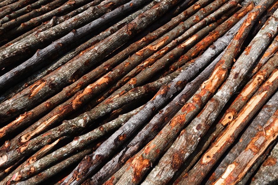
Stacking logs with the end grain facing upward or downward creates a natural barrier against rapid moisture loss. By placing a dry block or a piece of plywood on the top of each log, the exposed end grain is shielded from direct airflow, allowing the interior to dry at a more uniform rate
It cuts drying time
Standard Operating Procedure PDFs
Standard Operating Procedure PDFs provide a step‑by‑step framework for safely drying logs that have suffered water damage. The documents outline initial inspection, moisture‑meter calibration, and staging of logs in a controlled environment. They recommend using a calibrated moisture meter to confirm the target moisture content (typically 12–15 % for firewood). The SOPs detail the optimal stacking method: logs should be placed on a dry, level surface with the end grain protected by a plywood or concrete slab to slow rapid surface drying and reduce cracking. They also describe the use of solar kilns for large volumes, noting that a 30‑day cycle at 70 °F ambient temperature can bring logs to the desired moisture level while preserving grain integrity. For smaller batches, the SOPs advise conventional oven drying at 200 °F for 4–6 hours, with logs rotated every hour to ensure even drying. The PDFs include a monitoring schedule, advising daily checks of moisture content and visual inspection for signs of mold or split. They also provide a logbook template for recording date, moisture readings, and any corrective actions taken. Finally, the documents emphasize safety protocols, such as using fire‑resistant gloves, eye protection, and ensuring proper ventilation during kiln operation. By following these PDFs, woodworkers can achieve consistent, high‑quality results while minimizing waste and protecting the structural integrity of the logs. The PDF guides provide for moisture spikes.!! !!! !!